[#11] Deep Dive into Clustering (Part 1)
The k-Means algorithm and choosing the number of clusters

One of the main branches of machine learning is known as "unsupervised learning", whereby there are no labels on your training dataset. One thing that you can do with such a dataset is to cluster the data points to look for natural groupings within the data. Perhaps the most famous clustering algorithm is the k-Means algorithm.
A lot has been written about the k-Means algorithm, as it is perhaps the most famous unsupervised learning algorithm, so I am not going to dive into how the algorithm works (here is one video from Coursera).
Instead, I want to focus on one of the main issues that one has to address when one is running k-Means, and that is the issue of how many clusters are there in the dataset. As k-Means does not figure this out on its own, we must supply k-Means with the number of clusters to look for.
In subsequent posts in this series on clustering, I will look at alternatives to k-Means, particularly in scenarios where k-Means does not give ideal results, even when we do know the number of clusters beforehand.
You can find a Jupyter notebook with all of the code needed to generate the results below on GitHub.
Sample Data
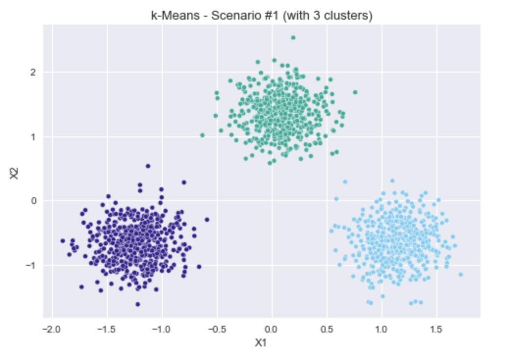
To generate sample data to work with, I used the make_blobs function in scikit-learn (sklearn.datasets.make_blobs). I designed the sample data so that visually it should be fairly obvious how many clusters there are, and then we can see how the k-Means clustering algorithm handles each one below.
Three scenarios (which are shown in the plots above):
Three simple, well-separated blobs.
The same three blobs from scenario #1, plus an additional blob very close to one of the existing ones (but all 4 are still visually separable).
The same three blobs from scenario #1, plus a fourth blob very far away.
How do we choose the number of clusters?
I will explore four options for determining the number of clusters:
The inertia parameter and the so-called "elbow plot"
The silhouette coefficient
The gap statistic
The prediction strength
Option 1: The “Elbow Plot”
This first option makes use of the inertia parameter, which is calculated as part of the k-Means algorithm itself. The inertia parameter is the sum of the squares of the distances of each point from its cluster center. Therefore, for the same dataset, the more clusters you have, the lower the inertia parameter is (the extreme case would be if you had as many clusters as data points and then the distance of each point from its cluster center would be zero and thus the inertia would be 0).
Therefore, one technique practitioners use is to plot the inertia versus the number of clusters (for the same dataset). Note that k-Means has to be re-run multiple times, once for each number of clusters that you want to consider. This plot of the inertia versus the number of clusters is referred to as the "elbow" plot because there should be a noticeable point where the inertia stops rapidly decreasing. This point should be the ideal number of clusters to use.
Option 2: The Silhouette Coefficient
The silhouette coefficient is calculated as follows:
The Silhouette Coefficient is calculated using the mean intra-cluster distance (
a) and the mean nearest-cluster distance (b) for each sample. The Silhouette Coefficient for a sample is(b - a) / max(a, b). To clarify,bis the distance between a sample and the nearest cluster that the sample is not a part of.Source: scikit-learn documentation1
In other words, this metric calculates how well each point has been clustered with 1 being a perfect clustering, 0 indicating the point in a region of overlap between two clusters, and -1 indicates that a point has been assigned to the wrong cluster.
One can then plot the average of this metric over all points versus the number of clusters. The number of clusters that gives the largest mean silhouette coefficient should give the ideal clustering.
Option 3: The Gap Statistic
The gap statistic method can be described as follows:
The gap statistic compares the total intracluster variation for different values of k with their expected values under null reference distribution of the data (i.e. a distribution with no obvious clustering). The reference dataset is generated using Monte Carlo simulations of the sampling process.
In other words, for each feature, or dimension, of the dataset, a uniform distribution of points is generated between the minimum and maximum values of that feature. The algorithm then finds which number of clusters gives the largest "gap" between the intracluster variation of the uniform dataset and the intracluster variation of the real data points.
To calculate the gap statistic, I use the gap statistic package2.
Option 4. The Prediction Strength
I came across this last method, the “prediction strength” in The Hundred-Page Machine Learning Book3. You can find a description there, as well as in this Medium article4.
Essentially, this method breaks the sample dataset into a training and test dataset, runs k-Means on both datasets, and essentially looks for consistent cluster labelling between the training and test sets.
The largest number of clusters that gives consistent cluster labelling is taken as the ideal number of clusters to use.
To calculate the prediction strength, I use a Python script provided here5.
k-Means Clustering for Scenario #1
The first scenario is three clear, separate, circular blobs of points, so it would be expected that all four options for choosing the number of clusters would return 3 as the result.
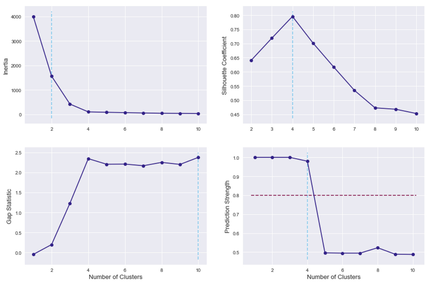
As a reminder, for inertia (in the top left), lower values are better, whereas higher values are better for the other three methods. In all metrics, the selection of 3 clusters clearly gives the best results.
k-Means Clustering for Scenario #2
For this scenario, I added a fourth blob that is very close to the upper blob from scenario #1. To my eye, these should be two separate blobs, but this might be where clustering can become a little subjective. If we tell k-Means that there are just 3 clusters, then, predictably, it creates one cluster from the two close-together blobs, and the other two original blobs are separate clusters.
With the silhouette coefficient and the prediction strength, 4 clusters is the clear choice. With the gap statistic, 4 clusters is also the prediction, although higher numbers of clusters also had fairly high scores.
With the “elbow” plot, my technique for automatically finding the elbow identifies the elbow at 3 clusters, although looking at the plot by eye, maybe I would pick out 4 clusters as the more obvious location of an “elbow”.
k-Means Clustering for Scenario #3
For this scenario, I added a fourth blob far away from the original three. Four clusters seems like the obvious number here, although, again, maybe some would argue it’s two clusters. When running k-Means with just two clusters, it gives the results I would expect, with the three original blobs as one cluster and the far-away blob as another cluster.
Again, the silhouette coefficient and the prediction strength show 4 clusters as the clear choice. With the gap statistic, the scores were fairly similar from 4 to 10 clusters, and the function I used for calculating the gap statistic predicted 10 clusters here. Looking at how k-Means performs the clustering when it is told to find 10 clusters for this dataset, the clustering doesn’t really make much sense. It is unclear why a clustering metric would give 10 clusters the same or higher score than 4 clusters in this scenario.
With the “elbow” plot, my technique for automatically finding the elbow identifies the elbow at 2 clusters, although looking at the plot by eye, again, maybe I would pick out 4 clusters as the more obvious location of an “elbow”.
Reviewing the Results
I explored here four techniques for automatically detecting the number of clusters in a dataset when using k-Means clustering. For each test, I used three or four circular blobs of points, where the points are distributed normally within the blobs.
The two techniques that consistently gave good results were the silhouette coefficient and the prediction strength.
Another important consideration is the runtime of the different techniques. Running just k-Means with 2000 data points with the cluster number already known took 44 ms on my computer. Checking 9 different cluster numbers took 490 ms for the elbow method, 1 second for the silhouette method, and 110 ms for the gap statistic method.
The prediction strength method took significantly longer, taking 21 seconds just to run it for two cluster numbers.
I will briefly summarize how each of the four techniques performed here.
Option 1: The “Elbow Plot”
The issue with the “elbow plot” is that when looking at it by eye, it may be easy to identify the “elbow” (at least in the test cases here), but it seems difficult to accurately pick-up the “elbow” location in an automated way.
Option 2: The Silhouette Coefficient
In the test cases here, using the number of clusters that gives the maximum silhouette coefficient seems to give accurate results, without slowing down the runtime as much as the prediction strength.
One potential downside of the silhouette coefficient is that it is undefined if there is only one cluster, so there is no way to consider the option of one cluster compared to two or more clusters. So, if you had a dataset that actually would be best clustered as just a single cluster, this method would not be able to pick-up on this.
Option 3: The Gap Statistic
This option sometimes gave different results, even for the "easy" case of Scenario #1, with three well-separated clusters. For Scenario #3, running the gap statistic algorithm multiple times gave estimates for the best cluster number ranging from 4 clusters to 10 clusters.
This lack of consistency is definitely a strike against this technique, even though it does seem to be the fastest one.
Option 4: The Prediction Strength
This option is very slow, at least using the code I found to calculate this metric (it took 20 seconds to check just two different cluster numbers, whereas the silhouette coefficient took just 1 second to check 9 different cluster numbers). Perhaps, it could be made a bit more efficient, but it is currently very expensive to check a large number of cluster numbers.
Also, the technique relies on choosing a threshold, which has been reported to be 0.8, for selecting the best number of clusters. In the "easy" case of Scenario #1 above, the selection of 6 clusters gives a prediction strength of 0.78, which is very close to 0.8. It would be interesting to know how strongly this threshold holds up in many different real-world scenarios.
Is There Another Option?
The common downside to all of these techniques is that they all require running k-Means multiple times, each time checking how good the clustering is. Is there an algorithm that figures out the number of clusters on its own, as part of the fitting process? I will explore this in a subsequent post!
Practical Data Science Tips
I will occasionally include here some random tips that are not always directly related to data science, but can help with some of the day-to-day tasks.
If you are using version control, in particular git, for your code, and you want to back up your repository, without using Github, or some other similar service, you can push your repository to a directory within your Dropbox or Tresorit (or whichever cloud storage provider you use). Each time you push to this directory, the repository gets backed up in your cloud storage.
You can find the instructions here.


